
August 2025
Introduction to Genome Assembly with Oxford Nanopore Sequencing
Welcome to the Workshop
Genome assembly represents one of the most fundamental and transformative processes in modern genomics, serving as the foundation for virtually all downstream genomic analyses. In this workshop, you will learn the essential principles and practical techniques for assembling genomes using Oxford Nanopore Technology (ONT) sequencing data, gaining hands-on experience with one of the most revolutionary sequencing platforms in contemporary biology.
The Critical Importance of Draft Genome Assemblies
Foundation of Genomic Understanding
Draft genome assemblies serve as the cornerstone of modern biological research, providing the essential framework for understanding life at its most fundamental level. A genome assembly is essentially a computational reconstruction of an organism's complete DNA sequence, assembled from millions of overlapping sequence fragments. While "draft" assemblies may not achieve the perfection of finished reference genomes, they provide invaluable insights that drive scientific discovery across multiple disciplines.
The importance of draft genomes extends far beyond academic curiosity. In medicine, genome assemblies enable the identification of disease-causing genetic variants, facilitate personalized treatment approaches, and accelerate drug discovery. Agricultural applications include crop improvement through the identification of beneficial traits and resistance genes. In evolutionary biology, comparative genomics using draft assemblies reveals the relationships between species and the mechanisms driving adaptation and speciation.
Democratizing Genomic Research
Draft genome assemblies have democratized genomic research by making genome sequencing accessible to laboratories worldwide. Unlike finished genomes, which require substantial time and computational resources, draft assemblies can be generated relatively quickly and cost-effectively while still providing sufficient quality for most research applications. This accessibility has led to an explosion in the number of sequenced genomes, with thousands of new species being sequenced annually.
The impact of this democratization cannot be overstated. Small research groups can now tackle questions that were previously the exclusive domain of large genome centers. This has led to breakthrough discoveries in non-model organisms, rare diseases, and microbial communities that would otherwise remain unstudied.
Enabling Personalized Medicine and Precision Agriculture
In clinical applications, draft genome assemblies of pathogens enable rapid identification and characterization during disease outbreaks. The COVID-19 pandemic demonstrated the critical importance of quick genome assembly capabilities, as researchers worldwide used draft assemblies to track viral evolution, identify variants of concern, and develop targeted interventions in near real-time.
Similarly, in agriculture, draft assemblies of crop plants and their associated microbiomes provide insights into plant health, stress resistance, and yield optimization. These assemblies enable breeders to make informed decisions about crop improvement and help farmers optimize growing conditions based on the genetic characteristics of their crops.
Oxford Nanopore Technology: Revolutionizing Genome Assembly
The Long-Read Advantage
Oxford Nanopore Technology has fundamentally transformed the landscape of genome assembly through its unique approach to DNA sequencing. Unlike traditional short-read sequencing technologies that produce fragments of 150-300 base pairs, ONT generates extraordinarily long reads that can span tens of thousands of base pairs, with some reads exceeding 100,000 base pairs in length.
This long-read capability addresses one of the most persistent challenges in genome assembly: repetitive sequences. Traditional short-read assemblies often struggle with repetitive elements, structural variants, and complex genomic regions, resulting in fragmented assemblies with gaps and misassemblies. ONT's long reads can span these problematic regions entirely, providing the contiguity necessary for high-quality assemblies.
Real-Time Sequencing and Portability
One of ONT's most revolutionary features is its real-time sequencing capability. Unlike other sequencing platforms that require hours or days to complete a run, ONT devices stream data continuously during sequencing. This enables researchers to monitor assembly quality in real-time and make informed decisions about when to stop sequencing, optimizing both time and cost.
The portability of ONT devices, particularly the MinION, has brought genomic sequencing capabilities to field stations, remote locations, and resource-limited settings. This portability has enabled groundbreaking research in biodiversity hotspots, rapid pathogen identification during outbreaks, and real-time monitoring of environmental samples.
Direct DNA Sequencing and Methylation Detection
ONT's nanopore sequencing technology directly measures native DNA molecules as they pass through biological nanopores, eliminating the need for amplification steps that can introduce bias. This direct approach preserves important epigenetic modifications, particularly DNA methylation, which plays crucial roles in gene regulation and development. The ability to simultaneously assemble genomes and characterize their epigenetic landscapes provides unprecedented insights into genome function.
The Perfect Synergy: ONT and Genome Assembly
Simplified Assembly Workflows
The combination of ONT's long reads and modern assembly algorithms has dramatically simplified genome assembly workflows. While short-read assemblies often require complex strategies involving multiple library types and careful parameter optimization, ONT assemblies can frequently be generated using straightforward approaches with minimal preprocessing.
Modern ONT assembly pipelines can transform raw sequencing data into high-quality draft assemblies in hours rather than days or weeks. This speed enables iterative approaches where researchers can quickly assess assembly quality and adjust sequencing strategies if needed.
Resolving Complex Genomic Features
ONT's long reads excel at resolving complex genomic features that have traditionally been challenging for genome assembly. These include structural variations, tandem repeats, centromeres, and highly variable regions such as immune system genes. The ability to accurately assemble these regions provides more complete and biologically meaningful genome representations.
Cost-Effective High-Quality Assemblies
The efficiency of ONT-based assembly workflows has made high-quality genome assembly more cost-effective than ever before. Researchers can often achieve draft assemblies suitable for most research purposes using a single ONT flow cell, dramatically reducing the cost per genome compared to traditional approaches.
Learning Objectives and Workshop Overview
Throughout this workshop, you will develop practical skills in handling ONT sequencing data, understanding quality metrics, and implementing assembly workflows. You will learn to evaluate assembly quality, identify potential issues, and optimize assembly parameters for different types of genomic data.
By the end of this workshop, you will understand how ONT's unique characteristics enable high-quality genome assemblies and how these assemblies serve as powerful tools for addressing diverse biological questions. You will be equipped with the knowledge and skills necessary to implement genome assembly projects in your own research, contributing to the expanding universe of genomic knowledge that continues to transform our understanding of life itself.
The skills you develop here will prepare you for the exciting frontier of genomics, where new discoveries await in every genome assembled and every question asked. Welcome to the world of genome assembly with Oxford Nanopore Technology – where the blueprint of life becomes accessible, interpretable, and transformative.
Workshop: 1KSA Genome Assembly
This handbook provides step-by-step instructions for performing de novo genome assembly using Oxford Nanopore Technology (ONT) sequencing data using the Flye assembler on the SAIAB High Performance Computer. The workshop is designed for individuals with minimal bioinformatics.
What You Will Learn
- Navigating the command line: Basic Linux commands, file navigation, and working with remote servers.
- Fundamentals of genome assembly: Understanding de novo assembly, its importance, and how ONT sequencing data is used in the process.
- Accessing and using SAIAB: How to log in, navigate the system, and configure your environment for genome assembly.
- Running the Flye assembler: Step-by-step instructions for assembling a genome, including input preparation, command execution, and parameter selection.
- Evaluating assembly quality: How to assess genome completeness, contiguity, and accuracy using tools such as QUAST and BUSCO.
- Troubleshooting common issues: Identifying and resolving problems related to read quality, assembly fragmentation, and computational errors.
Pre-requisites
SAIAB account & project access
Participants must have an active SAIAB account. If you don’t have an account or haven’t been granted project access, please reach out to SAIAB support well in advance to set this up.
- Basic command line knowledge
A basic understanding of command line operations is required for participants, including:
Navigating directories (cd, ls, pwd)
Viewing and editing files (nano, less, cat)/p>
Copying, moving, and removing files (cp, mv, rm)
Running basic shell commands (echo, grep, find)
Prerequisite training:
Participants must work through the SAIAB Introduction to Unix for Bioinformaticians.
Schedule
Day 1: Introduction & data preparation
09:00 – 09:30 | Welcome & workshop overview
Introduction to the 1KSA project
Goals and learning outcomes of the workshop
Overview of the workshop schedule
09:30 – 10:30 |Getting started & logging into the SAIAB
Computer setup
Logging into SAIAB via SSH
Navigating the command line
Linux refresher exercises
10:30 – 10:45 | Coffee Break
10:45 – 11:30 | Understanding the SAIAB setup & submitting jobs
Loading modules
Understanding the SLURM job scheduler
SLURM commands
Job script parameters
11:30 – 12:30 | Pipeline overview & download
Overview of pipeline steps
SAIAB setup
Clone the pipeline repository with the necessary scripts
Dependencies
12:30 – 13:30 | Lunch Break
13:30 – 15:00 | Running the pipeline
Data preparation
Running each step individually
Interpretation of results
15:00 – 15:15 | Break
15:15 – 16:30 | Running the pipeline
Running each step individually
Running the pipeline with a script
Interpretation of results
Day 2: Quality assessment & troubleshooting
09:00 – 10:30 | Evaluating assembly quality
Species Identification
Evaluating assembly quality and generating a report
Generate snail plots
10:30 – 10:45 | Coffee Break
10:45 – 12:30 | Troubleshooting common issues
Kmer-Analysis (no peaks detected)
Diagnosing poor assembly results (low coverage, fragmentation)
Addressing issues with read quality and contamination
Handling computational errors and resource limitations
Low BUSCO completeness: improving assembly quality
12:30 – 13:30 | Lunch Break
13:30 – 15:00 | Wrap-up & feedback
Q&A and feedback session
Getting started
# Terminal
These black coloured boxes are code blocks.
1. Accessing the SAIAB server
Logging into SAIAB via SSH
ssh username@lab417.saiab.ac.za                             #use your username and password
# You are on the login node
2. Linux & SLURM Basics
2.1 Essential Linux commands
pwd                  # print current directory
ls                   # list files
ls -lh               # list with sizes and permissions
cd /path/to/dir      # change directory
mkdir my_folder      # create a directory
cp file1 file2       # copy a file
mv file1 file2       # move or rename a file
cat file.txt         # print file contents
head -20 file.txt    # show first 20 lines
rm file.txt          # delete a file
2.2 Managing sessions with screen
Use screen to keep your work running after you disconnect from SSH.
# Start a new named session
screen -S workshop

# Detach (leaves session running in background)
Ctrl + A, then D

# List all sessions
screen -ls

# Reattach to a session
screen -r workshop
2.3 Understanding SLURM
The SAIAB cluster uses SLURM to schedule compute jobs. You submit a job to a queue; SLURM runs it when resources are free. Jobs are prioritised by wait time and fair-share usage. The only partition on SAIAB is agrp. If your job exceeds its requested time it will be killed automatically.
2.4 SLURM commands
| Command | Description |
|---|---|
squeue -u username |
View your queued and running jobs |
sbatch script.sh |
Submit a job script to the scheduler |
scancel 1133 |
Cancel job with ID 1133 |
srun --cpus-per-task=2 -t 0-6:30 --mem 10G --pty /bin/bash |
Start an interactive session (2 CPUs, 10 GB RAM, 6h30m) |
2.5 Job script example
Job parameters are set as #SBATCH lines at the top of a bash script.
#!/bin/bash
#SBATCH --partition=agrp          # queue to use
#SBATCH --time=14-00:00:00        # max runtime (days-hours:minutes:seconds)
#SBATCH --cpus-per-task=2         # CPUs per task
#SBATCH --mem=100G                 # RAM per node
#SBATCH --error=job.%J.err        # stderr log (%J = job ID)
#SBATCH --output=job.%J.out       # stdout log
#SBATCH --job-name=my_job         # name shown in squeue

# Your commands below:
bash master.sh /path/to/fastq/file
# Submit the script:
sbatch script.sh2.6 Setting up your environment
# 1. Start a screen session so work survives disconnection
screen -S workshop

# 2. Request an interactive compute node via SLURM
srun --cpus-per-task=2 -t 0-6:30 --mem 10G --pty /bin/bash

# 3. Activate the software environment
source /opt/miniconda3/bin/activate biotools

# 4. Confirm your job is running
squeue -u $USER
Once the biotools environment is active, check that every tool used in this workshop is available. Each line below should print a path; if any prints nothing, tell an instructor before you start.
# 5. Verify the workshop tools are installed
for tool in NanoFilt NanoPlot kmc flye minimap2 samtools racon busco quast nextflow; do
  printf '%-10s ' "$tool"; command -v "$tool" || echo "MISSING";
done
BlobTools (used for the snail plot near the end) lives in a separate btk environment. Check it like this — then switch back to biotools to continue:
# 6. Verify BlobTools in the btk environment
source /opt/miniconda3/bin/activate btk
command -v blobtools || echo "blobtools MISSING"
source /opt/miniconda3/bin/activate biotools
3. Pipeline overview and download
3.1 Overview of pipeline
The genome assembly pipeline is designed to process raw sequencing data into a polished, high-quality draft genome. Below, we outline the pipeline’s steps, their importance, and benchmarking metrics for evaluating their success.
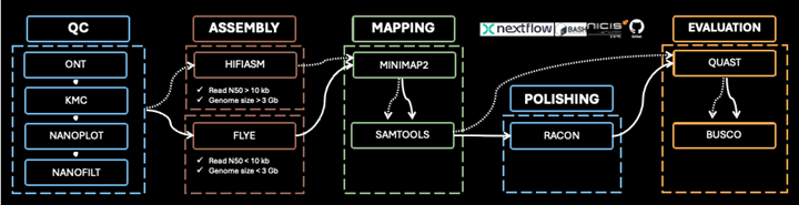
In this course we will run the 1KSA workflow step by step on the command line and in the end we will show how one can run it automatically as a pipeline using Nextflow.
Nextflow is a workflow management system designed specifically for computational pipelines, especially popular in bioinformatics and data science.
3.2 Clone the pipeline repository with the necessary scripts
# Navigate to your home folder
cd ~
# Copy the pipeline files to your directory
cp -r /opt/courses/ont_assembly_course/ .# Navigate inside the folder of the pipeline:
cd ont_assembly_course
# List what you have downloaded
ls -1 01_qc_and_trimming.nf
03_mapping.nf
04_polishing.nf
05_eval_final.nf
data
kmer-Analysis.sh
kmerPlot.R
master.sh
params.config
README.md
run_analysis.sh
run_flye.sh3.3 Dependencies:
# Download the BUSCO lineage folder
busco --download bacteria_odb10
# Make sure the download was completed:
ls ./busco_downloads/lineages/bacteria_odb10
It should return the following:
ancestral ancestral_variants dataset.cfg hmms info lengths_cutoff links_to_ODB10.txt refseq_db.faa.gz refseq_db.faa.gz.md5 scores_cutoffBUSCO uses a set of evolutionarily-informed expectations of gene content of near-universal single-copy orthologs to assess the completeness of genome assemblies, gene sets, and transcriptomes.
Running the pipeline
Data preparation
# Change to your working directory and the data folder
cd ont_assembly_course/Genome-Assembly-Pipeline-Nextflow/data
# Unzip files
gunzip -d escherichia_coli_data.fastq.gz
# List files in folder
ls -1
escherichia_coli_data.fastq# Move up to previous directory
cd ..K-mer Analysis
The primary goal of k-mer analysis is to evaluate the distribution of sequence fragments (k-mers) in raw sequencing data (Manekar and Sathe, 2018). This analysis provides insights into the quality of sequencing data, genome size estimation, sequencing coverage, and the complexity of the genome. It is a critical step in optimizing genome assembly processes, especially for de novo genome assemblies without reference genomes.
Genome size estimation: K-mer analysis provides an approximate estimate of the genome size based on k-mer frequencies, particularly useful for organisms without reference genomes.
Coverage assessment: Helps assess the sequencing depth and whether there is sufficient coverage for a reliable genome assembly.
Error detection: Identifies sequencing errors through over-represented or under-represented k-mers, which may indicate biases or library preparation issues.
Data complexity: Evaluates the complexity of the genome, including repetitive regions or unusual GC content, which impacts the assembly process.
K-mer distribution: A histogram representing k-mer frequencies. A well-defined peak indicates consistent coverage, while the absence of a peak may suggest insufficient coverage or sequencing issues.
Peak location: The position of the peak on the histogram reflects the estimated genome size. A high, sharp peak typically indicates accurate sequencing coverage.
K-mer depth (coverage): The height of the peak represents the sequencing depth. Adequate coverage (e.g., 50x–100x) ensures reliable assembly.
K-mer error rate: An excessive number of low-frequency k-mers can indicate sequencing errors or poor library preparation.
GC content: Confirms whether the genome’s GC content aligns with expected values, identifying potential sequencing biases.
K-mer size and cutoff values: Appropriate k-mer size and frequency cutoffs help filter out sequencing noise and improve assembly accuracy.
Two scripts are used for this step, which is included in the Genome-Assembly-Pipeline-Nextflow repository:
- kmer-analysis.sh
- kmerPlot.R (used by the first script)
This first script loads the necessary modules, calculates k-mer frequencies from a FASTQ file using KMC, generates a k-mer histogram, and runs an R script for k-mer frequency analysis on raw sequencing reads to estimate genome size, coverage, and ploidy.
Output files:
- total_number_bases.txt
- kmer21_histo.txt
- kmer21_K_mers.txt
- kmer21_K_mers.pdf
- kmer21_k_mers.png
Example of the kmer21_k_mers.png:
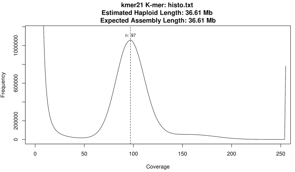
Key metrics from the plot
Estimated Haploid Length: 36.61 Mb
- This is the estimated genome size for a haploid version of your organism, inferred from the k-mer distribution.
Expected Assembly Length: 36.61 Mb
- This is the expected length of the genome assembly, often similar to the haploid length in diploid organisms without much variation or duplication.
Understanding the Plot
X-axis (Coverage):
- Represents how often each unique k-mer occurs in your sequencing data (i.e., sequencing depth or k-mer coverage).
Y-axis (Frequency):
- The number of k-mers that occur at each coverage level. Higher on the Y-axis means more k-mers with that specific coverage.
Peaks in the Histogram
Left Peak (Coverage ~1–30):
- Represents sequencing errors or low-frequency k-mers (likely from errors or rare variations).
- These are often filtered out during assembly.
Main Peak (Coverage ~97):
- Represents correct, high-confidence k-mers.
- The peak coverage (at 97x) indicates your average sequencing depth; this is very good coverage, suggesting high-quality sequencing data.
Right Tail (Coverage >150–250):
- Usually corresponds to repetitive regions (e.g., rRNA genes, repeats) that occur multiple times in the genome, leading to higher coverage.
Interpretation and Quality Insights
A sharp, well-defined main peak at coverage 97 suggests:
- Good sequencing quality.
- Sufficient coverage for a reliable genome assembly.
- Low noise from sequencing errors, since the left error peak is clearly separated from the main peak.
Genome Size Estimation Accuracy:
- The haploid length of 36.61 Mb is a reliable estimate, assuming your k-mer size and filtering settings were appropriate.
In summary, k-mer analysis acts as a quality checkpoint before genome assembly, ensuring that the sequencing data is sufficient, accurate, and free from major biases or errors. By interpreting the histogram and key metrics, researchers can optimize their assembly pipelines and improve the final genome reconstruction.
# Resume screen session (if you detached previously)
screen -r workshop
# Navigate to the Genome-Assembly-Pipeline-Nextflow working directory:
cd ont_assembly_course/Genome-Assembly-Pipeline-Nextflow # Run kmer analysis script
bash kmer-Analysis.sh data/escherichia_coli_data.fastq escherichia_coli
# Record genome coverage and size
less k_mers_Stats_escherichia_coli.txtescherichia_coli: k-mer=17
Total input bases 176565874
Peaks or Plateaus detected=1
Estimated 2n at?n
2n Genome Length=0.0049 Gb at 36 X Coverage
Expected Assembly Length if fully collapsed=0.0098 Gb at 18 X Coverage
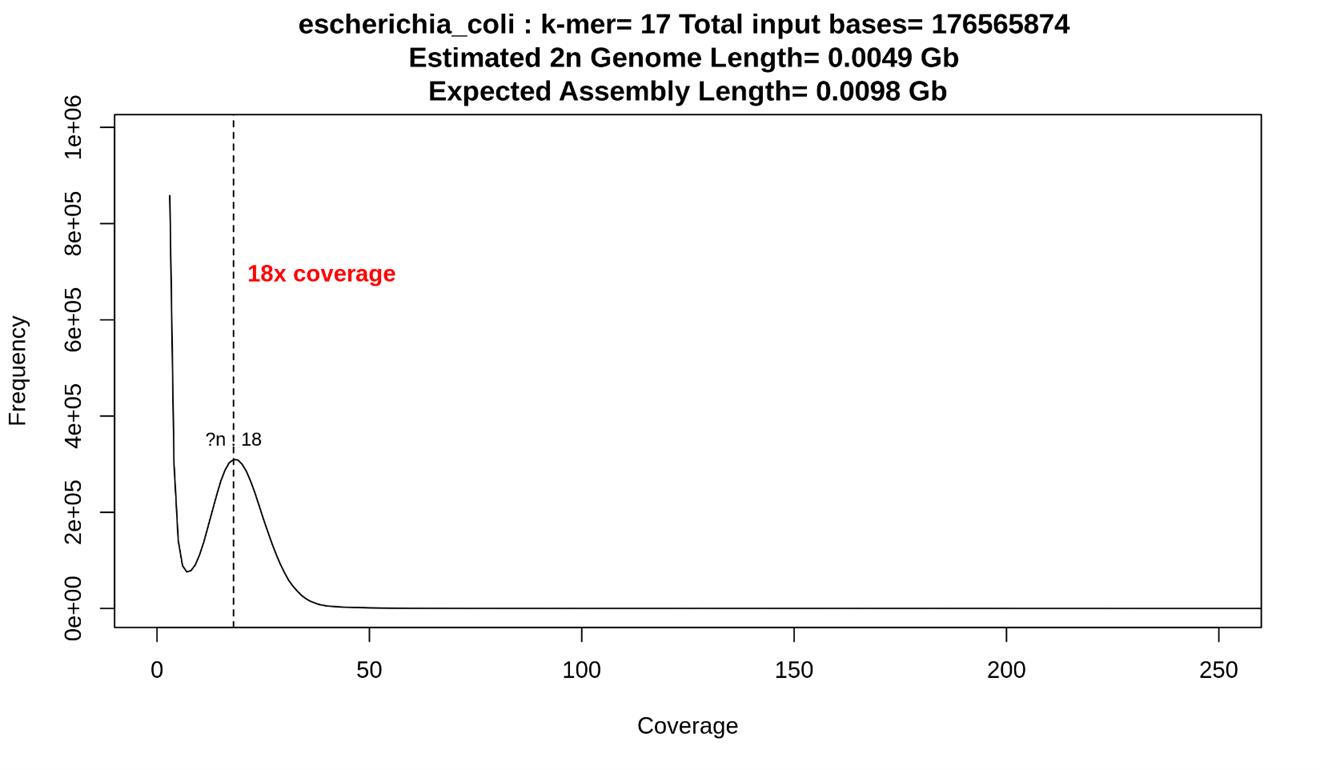
You will use the above output as input parameters when running the next steps.
# You can view the kmer plots in either png or .pdf format by opening the files in the SSH browser of Mobaxterm.Assessing Read Quality
Purpose:
To assess the quality of sequencing reads before any processing begins. High-quality raw reads are critical for successful downstream assembly and analysis.
Why It’s Done:
- Identifies sequencing errors, read length distribution, and data completeness.
- Helps detect any systematic issues with the sequencing run.
Important Metrics:
- Read N50: The length at which 50% of the total sequence data is contained in reads of equal or greater length.
- Average Read Length: Should align with the expected output of the sequencer (e.g., 10-20 kb for Oxford Nanopore).
- GC Content: Should reflect the expected range for the organism sequenced.
# Resume screen session
screen -r workshop
# Run NanoPlot on your fastq file:
NanoPlot -t 2 --fastq ./data/escherichia_coli_data.fastq --tsv_stats -o NanoPlot_CHECK_1 --no_static
# View the output file:
less ./NanoPlot_CHECK_1/NanoStats.txtMetrics dataset
number_of_reads 21452
number_of_bases 176565874.0
median_read_length 5178.5
mean_read_length 8230.7
read_length_stdev 9134.9
n50 15335.0
mean_qual 10.8
median_qual 11.8
longest_read_(with_Q):1 81743 (9.5)
longest_read_(with_Q):2 81102 (13.9)
longest_read_(with_Q):3 79307 (9.6)
longest_read_(with_Q):4 78113 (13.0)
longest_read_(with_Q):5 77919 (12.7)
highest_Q_read_(with_length):1 26.7 (37)
highest_Q_read_(with_length):2 25.6 (47)
highest_Q_read_(with_length):3 23.2 (91)
highest_Q_read_(with_length):4 22.9 (103)
highest_Q_read_(with_length):5 22.9 (49)
Reads >Q10: 15584 (72.6%) 133.0Mb
Reads >Q15: 2276 (10.6%) 17.7Mb
Reads >Q20: 27 (0.1%) 0.0Mb
Reads >Q25: 2 (0.0%) 0.0Mb
Reads >Q30: 0 (0.0%) 0.0Mb
To remove low-quality bases and adaptors from sequencing reads, ensuring that only high-confidence data is used for assembly.
Why It’s Done:
- Improves the accuracy of the assembly.
- Reduces computational burden by eliminating unnecessary or misleading data.
Important Metrics:
- Percentage of Reads Retained: Typically, >80% of reads should remain post-trimming.
- Mean Quality Score: Post-trim scores should exceed Q10 for base accuracy.
# Resume screen session
screen -r workshop
# Run NanoFilt on your fastq file:
mkdir trimmed_fastqNanoFilt -q 10 ./data/escherichia_coli_data.fastq > trimmed_fastq/escherichia_coli_data_trimmed.fastqPurpose:
To confirm the quality improvement of reads after trimming.
Why It’s Done:
- Verifies that trimming has effectively removed errors while retaining biologically meaningful data.
- Detects any anomalies introduced during the trimming process.
Important Metrics:
- Improved Mean Quality Score: An increase from raw read quality.
- Read Length Distribution: Consistency with expectations for trimmed reads.
# Run NanoPlot on your trimmed fastq file:
NanoPlot -t 1 --fastq ./trimmed_fastq/escherichia_coli_data_trimmed.fastq --tsv_stats -o NanoPlot_CHECK_2
# View the output file:
less ./NanoPlot_CHECK_2/NanoStats.txtMetrics dataset
number_of_reads 15584
number_of_bases 132950703.0
median_read_length 5443.0
mean_read_length 8531.2
read_length_stdev 9289.3
n50 15618.0
mean_qual 12.6
median_qual 12.8
longest_read_(with_Q):1 81102 (13.9)
longest_read_(with_Q):2 78113 (13.0)
longest_read_(with_Q):3 77919 (12.7)
longest_read_(with_Q):4 76635 (15.4)
longest_read_(with_Q):5 72781 (12.7)
highest_Q_read_(with_length):1 26.7 (37)
highest_Q_read_(with_length):2 25.6 (47)
highest_Q_read_(with_length):3 23.2 (91)
highest_Q_read_(with_length):4 22.9 (103)
highest_Q_read_(with_length):5 22.9 (49)
Reads >Q10: 15584 (100.0%) 133.0Mb
Reads >Q15: 2276 (14.6%) 17.7Mb
Reads >Q20: 27 (0.2%) 0.0Mb
Reads >Q25: 2 (0.0%) 0.0Mb
Reads >Q30: 0 (0.0%) 0.0Mb
Genome Assembly
De novo genome assembly reconstructs a genome from raw sequencing reads without using a reference genome. In order to do that, overlapping DNA sequences are used to build longer DNA sequences (contigs) and these contigs are arranged into a complete genome with the help of various statistical methods and algorithms.
Key Terms
- Reads: DNA sequences generated by the sequencer
- Contigs: Continuous sequences assembled from overlapping reads
- Scaffolds: Larger sequences created by linking contigs
- N50: A metric that represents assembly continuity
- BUSCO: A tool to assess assembly completeness
To generate a draft genome by assembling sequencing reads into contiguous sequences (contigs).
- Converts raw sequence reads into a coherent representation of the genome.
- Provides the structural foundation for downstream annotation and analysis.
- Assembly N50: Longer contigs indicate a more contiguous assembly.
- Total Assembly Size: Should approximate the expected genome size (e.g., 800 Mb).
- Number of Contigs: Fewer contigs suggest a more complete assembly.
# Resume screen session
screen -r workshop
# Ensure that the ont conda environment has been activated
source /opt/miniconda3/bin/activate biotools # Run Flye on the trimmed fastq file
# Value for --asm-coverage and estimated genome size –g is obtained from kmer analysis
flye --nano-raw trimmed_fastq/escherichia_coli_data_trimmed.fastq -o assembly --asm-coverage 18 -g 0.01g -t 2# View the output file:
tail ./assembly/flye.logExample INFO: Assembly statistics:
Total length: 5101716
Fragments: 6
Fragments N50: 4862946
Largest frg: 4862946
Scaffolds: 0
Mean coverage: 24
Mapping and Polishing
Genome assembly produces a draft — a best-guess reconstruction from overlapping reads. This draft contains errors: insertions, deletions, and substitutions introduced by the sequencer. Mapping and polishing correct these errors using the original reads as evidence.
Why map reads back to the assembly?
After assembly, the raw reads are aligned back to the draft genome. This shows exactly where reads agree with the assembly and where they disagree. Regions with low coverage or many mismatches flag potential misassemblies. The alignment file (SAM) is also the input for polishing.
- Alignment rate — aim for >95% of reads mapping. Lower rates suggest the assembly is missing sequence or reads are contaminated.
- Coverage depth — should match the expected sequencing depth (e.g., 30x). Regions with very low coverage are unreliable.
We use minimap2 for mapping. It is fast, handles long noisy ONT reads, and outputs a SAM file.
# Map the reads using minimap2
minimap2 -ax map-ont -t 2 ./assembly/assembly.fasta ./trimmed_fastq/escherichia_coli_data_trimmed.fastq > escherichia_coli.sam
Why polish?
ONT reads have a raw base-calling error rate of ~5-10%. Even after assembly, the consensus sequence retains some of these errors. Polishing uses the read alignments to vote on the correct base at each position, replacing draft errors with the most supported base call.
- Polishing iterations — typically 1-3 rounds. Each round uses the previous polished assembly as the new reference. Diminishing returns after 3 rounds.
- Expected improvement — error rate drops significantly after the first round; BUSCO completeness and QUAST metrics should both improve.
We use Racon for polishing. It is lightweight, works directly with minimap2 SAM output, and is well-suited to ONT data.
# Polish the assembly with Racon
mkdir Racon_results
racon -m 3 -x -5 -g -4 -w 500 -t 2 ./trimmed_fastq/escherichia_coli_data_trimmed.fastq escherichia_coli.sam assembly/assembly.fasta > ./Racon_results/Racon_polished.fasta
Genome Assembly Evaluation
Assembly evaluation answers the question: is this genome good enough to use? Raw assembly and polishing steps can introduce errors, leave gaps, or produce fragmented contigs. Evaluation catches these problems before downstream analysis (annotation, comparative genomics, publication).
Two complementary tools are used:
- QUAST — measures structural quality: number of contigs, total length, N50, and largest contig. Tells you whether the assembly is contiguous and the right size.
- BUSCO — measures biological completeness by checking for the presence of conserved single-copy genes expected in the organism's lineage. A score >95% complete indicates a high-quality assembly.
Run both after polishing. QUAST flags fragmentation; BUSCO flags missing gene content. Together they give a full picture of assembly quality.
# Run BUSCO on the polished assembly:busco -m genome -i ./Racon_results/Racon_polished.fasta -o Busco_outputs -l bacteria_odb10 --download_path ./busco_downloads --metaeuk_parameters METAEUK_PARAMETERS --offline# View the output file:
less ./Busco_outputs/short_summary.specific.bacteria_odb10.Busco_outputs.txt# BUSCO version is: 6.0.0
# The lineage dataset is: bacteria_odb10 (Creation date: 2024-01-08, number of genomes: 4085, number of BUSCOs: 124)
# Summarized benchmarking in BUSCO notation for file /home/evilliers/work/ont_assembly_course/Genome-Assembly-Pipeline-Nextflow/Racon_results/Racon_polished.fasta
# BUSCO was run in mode: prok_genome_prod
# Gene predictor used: prodigal
***** Results: *****
C:99.2%[S:99.2%,D:0.0%],F:0.8%,M:0.0%,n:124
123 Complete BUSCOs (C)
123 Complete and single-copy BUSCOs (S)
0 Complete and duplicated BUSCOs (D)
1 Fragmented BUSCOs (F)
0 Missing BUSCOs (M)
124 Total BUSCO groups searched
Assembly Statistics:
6 Number of scaffolds
6 Number of contigs
5103316 Total length
0.000% Percent gaps
4 Mbp Scaffold N50
4 Mbp Contigs N50
Dependencies and versions:
hmmsearch: 3.4
bbtools: None
prodigal: 2.6.3
To validate the final genome assembly’s quality and structural accuracy.
- Ensures the genome meets the standards for downstream analysis.
- Provides a final report for benchmarking and publication.
- Improved N50 and Contig Sizes: Indicate a high-quality, contiguous assembly.
- Genome Fraction: Should align closely with the expected genome size.
QUAST (Quality Assessment Tool for Genome Assemblies) evaluates assembly quality without a reference genome. It reports key metrics: number of contigs, total assembly length, N50 (the length at which 50% of the assembly is contained in contigs of that size or longer), and largest contig. A good assembly has few contigs, high N50, and total length close to the expected genome size.
# Run QUAST on the polished assembly file:quast.py -t 2 -o Quast_output --gene-finding ./Racon_results/Racon_polished.fasta --fragmented
# View the output file:
less ./Quast_output/report.txt
All statistics are based on contigs of size >= 500 bp, unless otherwise noted (e.g., "# contigs (>= 0 bp)" and "Total length (>= 0 bp)" include all contigs).
Assembly escherichia_coli_Racon_polished
# contigs (>= 0 bp) 6
# contigs (>= 1000 bp) 6
# contigs (>= 5000 bp) 6
# contigs (>= 10000 bp) 4
# contigs (>= 25000 bp) 3
# contigs (>= 50000 bp) 3
Total length (>= 0 bp) 5103316
Total length (>= 1000 bp) 5103316
Total length (>= 5000 bp) 5103316
Total length (>= 10000 bp) 5084379
Total length (>= 25000 bp) 5067109
Total length (>= 50000 bp) 5067109
# contigs 6
Largest contig 4864756
Total length 5103316
GC (%) 50.83
N50 4864756
N90 4864756
auN 4641540.1
L50 1
L90 1
# N's per 100 kbp 0.00
Run the entire pipeline in one script
The 1KSA pipeline to perform de novo genome assembly with Oxford Nanopore long-read sequencing data has been implemented in Nextflow, a workflow management system designed specifically for computational pipelines, especially popular in bioinformatics and data science.
# Open and edit the params.config file
nano params.config
Change the following path and values:
# File: params.configspecies_name='1ksa_test' # Change species_name
assembler='flye' # Options: 'flye' or 'hifiasm'# Shared parameters
threads=2
LINEAGE='bacteria_odb10' #Mandatory BUSCO lineage (Other options: insecta_odb10, viridiplantae_odb10)# Flye-specific parameters (mandatory)
genome_size='0.0098g' # Mandatory genome size - adjust to the values obtained from the k-mer analysis
flye_coverage=18 # Mandatory coverage - adjust to the values obtained from the k-mer analysis
flye_read_type='nano-raw' # Default read type (can change to nano-hq for Q15 reads)# Save the script:
^X # Exit
y # Confirm Save
Enter The script master.sh is calling the different nextflow scripts for the analysis:
01_qc_and_trimming.nf
03_mapping.nf
04_polishing.nf
05_eval_final.nf
# Create a SLURM job script:
nano name_of_your_script_1.sh                          #change the name of the script
# Copy and paste the following
#!/bin/bash
#SBATCH --partition=agrp
#SBATCH --time=12:00:00
#SBATCH -N 1 # Nodes
#SBATCH -n 1 # Tasks
#SBATCH --cpus-per-task=2
#SBATCH --mem 100G
#SBATCH --error=/home/username/flye_stderr.%J.txt
#SBATCH --output=/home/username/flye_stdout.%J.txt
#SBATCH --mail-user=username@gmail.com
#SBATCH --mail-type=ALL
#SBATCH --job-name=1ksa_test_flyecd /path/to/folder/with/species/fastq/files/Genome-Assembly-Pipeline-Nextflow #change pathbash master.sh ./data/escherichia_coli_data.fastq## Save and Exit
^X # Exit
y # Confirm Save
Enter ## Submit SLURM job script
sbatch name_of_your_script_1.shResults from the bash script is saved to the folder ./results. These results can be summarized with the following script.
Evaluating assembly quality and generating a report
# Create a script:
nano generate_report.sh
# Copy and paste the following
#!/bin/bash
set -euo pipefail
# === USER INPUT ===
species_name="species_name" # Change species name (same as the species_name in params.config)
cd /path/to/results # Change to actual results folder
################################################################################
# PART 1 — SAMTOOLS PROCESSING
################################################################################
echo "=== PART 1: SAMTOOLS ==="
if [[ ! -f ./sam_file/${species_name}.sam ]]; then
echo "❌ ${species_name}.sam not found in ./sam_file/"
exit 1
fi
# Sort SAM → BAM
if [[ ! -f ./sam_file/${species_name}_sorted.bam ]]; then
echo "▶️ Sorting SAM..."
samtools view -bS ./sam_file/${species_name}.sam | \
samtools sort -o ./sam_file/${species_name}_sorted.bam
else
echo "✅ Sorted BAM already exists"
fi
# Coverage
if [[ ! -f ./sam_file/minimap2_coverage.txt ]]; then
echo "▶️ Calculating depth coverage..."
samtools depth ./sam_file/${species_name}_sorted.bam |
awk '{sum+=$3} END { print "Average = ",sum/NR}' \
> ./sam_file/minimap2_coverage.txt
else
echo "✅ Coverage already calculated"
fi
# Stats
if [[ ! -f ./sam_file/sam_stats.txt ]]; then
echo "▶️ Generating SAM stats..."
samtools stats ./sam_file/${species_name}_sorted.bam |
grep ^SN | cut -f 2- > ./sam_file/sam_stats.txt
else
echo "✅ SAM stats already exist"
fi
################################################################################
# PART 2 — Detect Assembler + Handle Coverage
################################################################################
echo "=== PART 2: Assembler Detection ==="
assembler=""
if [[ -d ./Flye_results ]]; then
assembler="flye"
elif [[ -d ./Hifiasm_results ]]; then
assembler="hifiasm"
fi
if [[ "$assembler" == "flye" ]]; then
echo "🔎 Flye assembly detected — extracting mean coverage..."
OUTPUT_FILE="${species_name}_flye_mean_coverage.txt"
> "$OUTPUT_FILE"
for logfile in $(find ./Flye_results -type f -name "flye.log"); do
mean_cov=$(grep "Mean coverage:" "$logfile" | awk '{print $3}')
[[ -n "$mean_cov" ]] && echo "$logfile: $mean_cov" >> "$OUTPUT_FILE"
done
elif [[ "$assembler" == "hifiasm" ]]; then
echo "🔎 Hifiasm assembly detected — no flye.log coverage to extract."
else
echo "⚠️ No assembler results directory found."
fi
################################################################################
# PART 3 — Collect Key Outputs
################################################################################
echo "=== PART 3: Collect Outputs ==="
mkdir -p "${species_name}" "${species_name}_other_results_outputs"
# NanoPlot results
mv ./nanoplot_before_trim/NanoPlot_CHECK_1/NanoStats.txt "${species_name}_NanoStats_before_trim.txt" 2>/dev/null || true
mv ./nanoplot_before_trim/NanoPlot_CHECK_1/NanoPlot-report.html "${species_name}_NanoPlot_before_trim.html" 2>/dev/null || true
mv ./nanoplot_after_trim/NanoPlot_CHECK_2/NanoStats.txt "${species_name}_NanoStats_after_trim.txt" 2>/dev/null || true
mv ./nanoplot_after_trim/NanoPlot_CHECK_2/NanoPlot-report.html "${species_name}_NanoPlot_after_trim.html" 2>/dev/null || true
# Trimmed FASTQ
mv ./trimmed_fastq/${species_name}.trimmed.fastq ./"${species_name}" 2>/dev/null || true
# Assemblies
if [[ "$assembler" == "flye" ]]; then
mv ./Flye_results/${species_name}_assembly.fasta ./"${species_name}/${species_name}_flye_assembly.fasta" 2>/dev/null || true
mv ./Racon_results/${species_name}_Racon_polished.fasta ./"${species_name}/${species_name}_racon_polished.fasta" 2>/dev/null || true
elif [[ "$assembler" == "hifiasm" ]]; then
mv ./Hifiasm_results/${species_name}_ctg.fasta ./"${species_name}/${species_name}_hifiasm_assembly.fasta" 2>/dev/null || true
fi
# BUSCO + QUAST
mv ./Busco_results/Busco_output/short_summary.specific.*.txt "${species_name}_busco_summary.txt" 2>/dev/null || true
mv ./quast_report/Quast_result/report.txt "${species_name}_quast_report.txt" 2>/dev/null || true
# Coverage + stats
mv ./sam_file/minimap2_coverage.txt "${species_name}_minimap2_coverage.txt"
mv ./sam_file/sam_stats.txt "${species_name}_sam_stats.txt"
################################################################################
# PART 4 — Compile Final Report
################################################################################
echo "=== PART 4: Final Report ==="
ordered_files=(
"${species_name}_kmer_total_number_bases.txt"
"${species_name}_kmer_cov_size.txt"
"${species_name}_NanoStats_before_trim.txt"
"${species_name}_NanoStats_after_trim.txt"
"${species_name}_minimap2_coverage.txt"
"${species_name}_sam_stats.txt"
"${species_name}_quast_report.txt"
"${species_name}_busco_summary.txt"
)
[[ -f "${species_name}_flye_mean_coverage.txt" ]] && ordered_files+=("${species_name}_flye_mean_coverage.txt")
report="${species_name}_report.txt"
{
echo "${species_name^} Assembly Report for RedCap"
echo "Generated on: $(date)"
echo -e "\n========================================\n"
for file in "${ordered_files[@]}"; do
if [[ -f "$file" ]]; then
echo "========== $file =========="
cat "$file"
echo -e "\n\n"
fi
done
} > "$report"
echo "✅ Report generated: $report"
################################################################################
# PART 5 — Organize Output Folders
################################################################################
echo "=== PART 5: Organizing Outputs ==="
mv *_NanoStats_before_trim.txt *_NanoStats_after_trim.txt *_NanoPlot_*.html "${species_name}" 2>/dev/null || true
mv "${species_name}"_busco_summary.txt "${species_name}" 2>/dev/null || true
mv "${species_name}"_quast_report.txt "${species_name}" 2>/dev/null || true
mv "${species_name}_minimap2_coverage.txt" "${species_name}_other_results_outputs" 2>/dev/null || true
mv "${species_name}_sam_stats.txt" "${species_name}_other_results_outputs" 2>/dev/null || true
mv "${species_name}_flye_mean_coverage.txt" "${species_name}_other_results_outputs" 2>/dev/null || true
mv nanoplot_before_trim nanoplot_after_trim quast_report Busco_results trimmed_fastq sam_file \
Flye_results Racon_results Hifiasm_results "${species_name}_other_results_outputs" 2>/dev/null || true
echo "🎉 All done!"Generate snail plots
BlobTools is a bioinformatics software package designed for visualizing and analyzing genome assemblies, particularly for quality control and contamination detection. The following commands will generate a visual summary of the assembly.
BlobTools lives in its own btk environment, so activate it before running the blobtools commands below. The samtools step still uses biotools.
# Convert sam file to bam file format and sort and index (biotools)
samtools view -@ 2 -b escherichia_coli.sam| samtools sort -@ 2 -o escherichia_coli_sorted.bam && samtools index -c escherichia_coli_sorted.bam
# Switch to the BlobTools environment
source /opt/miniconda3/bin/activate btk
# Create blobtools dataset from assembly
blobtools create --fasta Racon_results/Racon_polished.fasta escherichia_coli
# Add read coverage plot
blobtools add --cov escherichia_coli_sorted.bam --taxdump /data/db/taxdump/ escherichia_coli# Add busco results
blobtools add --busco Busco_outputs/run_bacteria_odb10/full_table.tsv escherichia_coli# Run blobtools view to generate a snail plot
blobtools view --plot --view snail escherichia_coli
# Switch back to biotools for the remaining steps
source /opt/miniconda3/bin/activate biotoolsDownload the escherichia_coli.snail.png file to your local device or open it up using the MobaXterm file viewer.
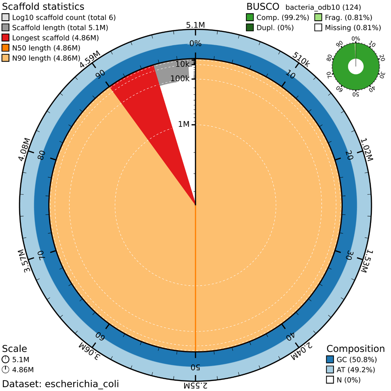
Assembly Statistics (Concentric Rings)
The data set used is a smaller version of a larger genome project to enable participants to generate an assembly during the course duration.
Scaffold Statistics
Total scaffolds: 6 (very low - good!)
Total length: 5.1 Mb (typical for E. coli ~4.6-5.5 Mb)
Longest scaffold: 4.86 Mb (represents ~95% of the genome)
N50 = N90 = 4.86 Mb (extremely high contiguity!)
BUSCO Results: Outstanding
Complete BUSCOs: 99.2% (123/124 genes) ✅
Duplicated: 0% (no contamination) ✅
Fragmented: 0.81% (1 gene partially found)
Missing: 0.81% (1 gene not found)
Key Insights
Highly contiguous assembly: One major contig (~4.86 Mb) contains almost the entire genome
Minimal fragmentation: Only 6 scaffolds total
No contamination: 0% duplicated BUSCOs
Proper GC content: 50.8% GC is typical for E. coli
Clean assembly: 0% Ns (no gaps)
Visual Elements
Large orange area: Main chromosome (4.86 Mb)
Small red wedge: Longest scaffold marker
Blue rings: Smaller scaffolds/contigs
Minimal fragmentation: Very few small pieces
The genome assembly pipeline is a meticulous process that transforms raw sequencing data into a polished draft genome. Each step is carefully designed to ensure the final assembly is accurate, complete, and ready for biological interpretation.
Troubleshooting common issues
1. “No Peaks or Plateaus Detected” in K-mer Analysis
If the k-mer histogram does not show a clear peak or plateau:
Possible Causes:
- Insufficient or excessive sequencing data, leading to noisy or flattened histograms.
- Poor-quality reads or contamination obscuring the true k-mer distribution.
Solution:
- Ensure balanced coverage: Both too little and too much data can cause problems. In one case with a fungal genome, downsampling excessively large datasets improved peak clarity and genome size estimation. (You can use seqtk to subsample a percentage of the reads).
- seqtk sample -s42 input.fastq 0.1 > subsampled.fastq
- -s42: Sets a random seed (change the number to get different subsamples).
- 0.1: Keeps 10% of the reads (adjust as needed).
- input.fastq: Your original FASTQ file.
- subsampled.fastq: Output file with the downsampled reads.
- Why it’s unbiased? Uses uniform random sampling while preserving diversity.
- Check read quality with FastQC and remove low-quality reads or adapters.
- Verify appropriate k-mer size (e.g., k=21) for your genome.
- If contamination is suspected, use tools like Kraken or FastQ Screen to assess and clean your dataset.
2. Diagnosing poor assembly results (low coverage, fragmentation)
Common symptoms include low N50, fragmentation, unexpected assembly size, or low genome completeness.
Possible Causes:
- Low coverage leading to incomplete assemblies.
- Low BUSCO completeness scores (e.g., <90%) suggests missing or fragmented conserved genes.
- Assembly size significantly smaller or larger than estimated genome size.
- High number of short contigs or scaffolds.
Solution:
- Increase sequencing depth.
- Use assemblers optimized for your read type and genome complexity (Figure 3).
- Pre-process data to remove adapters, contaminants, and low-quality reads.
- Ensure sufficient and balanced coverage (typically 30–60x for short reads, 20x for long reads).
- Re-evaluate read quality and trimming steps.
- Consider alternative assemblers or adjust parameters (e.g., error correction, minimum contig length).
- Assess for contamination affecting assembly with tools like BlobTools
Figure 3: Recommended Nanopore assembly strategies based on read length N50.
3. Addressing issues with read quality and contamination
Poor-quality reads or contamination can skew k-mer distributions and assembly.
Indicators: Excess low-frequency k-mers, unexpected peaks, or unusually high GC content.
Solution:
- Perform thorough quality trimming (e.g., with Trimmomatic, fastp).
- Remove contaminants using tools like Kraken or DecontaMiner.
- Evaluate GC content and coverage plots to identify anomalies.
4. Handling computational errors and resource limitations
K-mer counting and assembly are resource-intensive, especially with large genomes.
Common Errors: Job failures, memory limits exceeded, or storage issues.
Solution:
- Use a SAIAB queue with higher RAM and more cores to accommodate large-genome assemblies (bigmem queue; see under Bigmem queue on the SAIAB in the Appendix).
- Optimize job scheduling by monitoring resource usage and adjusting memory and core requests via PBS.
- Downsample input data where appropriate to reduce computational load without compromising assembly quality.
- Increase quality thresholds during trimming and filtering to improve data quality and minimize unnecessary processing.
- Use efficient tools like KMC for k-mer counting while fine-tuning parameters for memory efficiency.
- Modify workflow strategies by splitting large jobs, implementing checkpointing, or restructuring pipelines for better resource management.
5. Low BUSCO completeness: improving assembly quality
Certain genomes, such as the Western Leopard Toad, can be highly complex due to repetitive regions, high heterozygosity, or structural variation. Despite using Oxford Nanopore (ONT) long-read sequencing, assemblies may still show low BUSCO completeness due to fragmentation or missing genes.
1. If the assembly is fragmented (many short contigs)
Cause: Even with ONT long reads, assembly fragmentation can occur if reads are too short, error rates are high, or repeats are unresolved.
Solution:
Increase read length (N50) by optimizing library prep (e.g., high-molecular-weight DNA extraction, size selection).
Use higher-coverage data (e.g., ≥30x) to improve consensus accuracy and contiguity.
Experiment with alternative assemblers (e.g., Hifiasm, Flye, NextDenovo) to handle complex regions better.
Result: Longer, more contiguous scaffolds improve BUSCO scores by recovering full-length genes.
2. If the assembly is smaller than expected genome size
Cause: Insufficient coverage or filtering out of heterozygous/duplicated regions can result in missing genomic content.
Solution:
Increase sequencing depth to ≥20x–30x to ensure full genome representation.
Evaluate assembly parameters, some assemblers may collapse repeats or filter heterozygous regions, leading to underrepresentation.
Check for excessive read filtering/trimming, retaining more reads (even slightly lower quality) can help recover missing sequences.
Result: A more complete genome reconstruction with improved gene recovery.
3. Prioritizing longer Sequencing N50 vs. higher coverage of shorter reads
Tradeoff:
Longer N50 sequences improve contiguity and can resolve complex structures.
Higher coverage with shorter N50 reads can improve consensus accuracy and fill in missing regions.
Recommended Approach:
Aim for a balance, longer reads (>50 kb where possible) with sufficient coverage (≥20x) for complex genomes. Consider sequencing with two flow cells, using fragmented and non-fragmented DNA respectively.
If coverage is limited, focus on maximizing read length rather than accumulating more short reads.
Consider additional polishing (e.g., Medaka, Racon) to refine base accuracy post-assembly.
Result: Improved BUSCO completeness through better-contiguous and high-accuracy assembly.
Appendices
Genome assembly pipeline parameters
| Tool | Parameter Description | Parameter Flag | Value/Notes |
|---|---|---|---|
| NanoFilt | Quality | -q | 10 |
| Minimum read length | -l | 1000 | |
| Flye | ONT regular reads (Q>10) | --nano-raw | |
| ONT high-quality reads (Q>15) | --nano-hq | ||
| Threads | -t | 15 | |
| Reduced coverage | --asm-coverage | (k-mer analysis) e.g. 36 | |
| Genome size | -g | (k-mer analysis) e.g. 2.4g | |
| Racon | Match | -m | 3 |
| Mismatch | -x | -5 | |
| Gap | -g | -4 | |
| Window length | -w | 500 | |
| Threads | -t | 15 | |
| BUSCO | Database | -l | eukaryota_odb10 |
| Mode | -m | genome | |
| Metaeuk gene predictor | --metaeuk_parameters | METAEUK_PARAMETERS --offline |
Glossary
A
- Assembly (Genome Assembly): The process of reconstructing a complete genome sequence from smaller DNA sequence fragments.
- Adaptive Traits: Genetic features that enhance an organism's ability to survive and reproduce in specific environments. These traits may evolve due to natural selection and can be studied through comparative genomics.
- Annotation (Genome Annotation): The process of identifying and labeling functional elements in a genome, such as protein-coding genes, non-coding regions, and regulatory elements, often through sequence comparison with known genes.
- Amino Acid: The building blocks of proteins, coded by DNA sequences, which link together in chains to form proteins.
- Antimicrobial Resistance (AMR): The ability of microorganisms to resist the effects of drugs that once killed them or inhibited their growth, posing a serious threat to public health.
B
- Batch Job: A non-interactive job that runs on a high-performance computing (HPC) system when resources become available.
- Bigmem Queue: A SAIAB queue with high memory resources (1 TB RAM) used for memory-intensive tasks such as genome assembly.
- BUSCO (Benchmarking Universal Single-Copy Orthologs): A tool used to assess genome assembly completeness by comparing it to a database of conserved genes.
C
- SAIAB (Centre for High-Performance Computing): South Africa’s national supercomputing facility.
- Concatenation: The process of merging multiple files into a single file, e.g., combining multiple FASTQ files into one.
- Contigs: Continuous sequences assembled from overlapping reads.
- Coverage (Sequencing Coverage): The average number of times each nucleotide in a genome is sequenced, affecting accuracy and completeness.
- Contigs: Continuous sequences of DNA that result from the assembly of smaller sequencing reads. Contigs are used to build the larger genome assembly.
- Comparative Genomics: The field that compares the genomes of different species to understand their evolutionary history, functional genes, and adaptations to the environment.
D
- Detached Screen Session: A process running in the background after disconnecting from an SSH session, which can later be resumed.
- Draft Genome Assembly: A preliminary genome sequence generated from raw DNA sequencing data. While it may be incomplete or contain errors, it serves as the foundation for further analysis, including genome annotation and population genetics studies.
E
- Error Detection (K-mer Analysis): Identifying sequencing errors based on abnormal k-mer frequency distributions.
- Expected Assembly Length: The anticipated genome size after the assembly process, estimated from k-mer analysis.
- Evolutionary Relationships: The connections between different species based on shared ancestry. These are often studied using comparative genomics, which compares genetic sequences to understand the evolutionary history of organisms.
F
- FASTA File: A text file format that stores nucleotide or protein sequences without quality scores. Each sequence is represented by a header line (starting with >), followed by the sequence on the next lines.
- FASTQ File: A text file format that stores raw sequencing reads and their quality scores.
- Fairshare (SLURM): A priority adjustment system that ensures equal distribution of SAIAB computing resources among users.
- Flye: A genome assembler specifically designed for long-read sequencing technologies like Oxford Nanopore.
- Functional Genomics: The study of gene functions and their interactions, often using genome sequencing data.
G
- GC Content: The percentage of guanine (G) and cytosine (C) bases in a DNA sequence, used to evaluate sequencing quality.
- Genome Size Estimation: The process of predicting the total size of a genome using k-mer frequency distributions.
- grep: A command-line utility used to search text within files, often used to filter job queue information in SAIAB.
H
- Haploid Length (Estimated Haploid Length): The predicted genome size assuming a single set of chromosomes, calculated using k-mer analysis.
- Histogram (K-mer Histogram): A graphical representation of k-mer frequency distribution, helping assess sequencing quality.
- High-Performance Computing (HPC): The use of powerful computers to process complex tasks, such as genome assembly.
I
- Interactive Job: A real-time session on the SAIAB system that allows users to execute commands directly, often used for debugging.
- Inbreeding: Mating between closely related individuals, which can lead to a higher frequency of deleterious recessive traits. Studying inbreeding levels in populations is important for conservation biology.
K
- K-mer: A sequence of ‘k’ nucleotides used to analyze sequencing data and estimate genome size.
- K-mer Analysis: A computational approach to evaluate sequencing data quality, estimate genome size, and detect sequencing errors.
- K-mer Coverage: The number of times a specific k-mer appears in the dataset, used to infer sequencing depth.
L
- Lengau: The SAIAB supercomputer, accessed via SSH for computational tasks.
- Lineage Folder (BUSCO Lineage Folder): A reference dataset used by BUSCO to assess genome completeness.
M
- Module (Environment Module): A system that allows users to load and unload software packages dynamically on SAIAB.
- mpiprocs: The number of MPI (Message Passing Interface) processes allocated per node in a job submission.
- Metagenomics: The study of genetic material recovered directly from environmental samples, useful for understanding microbial diversity and function.
N
- N50: A metric that represents assembly continuity. It is the length of the shortest sequence in the largest group of sequences that together make up at least 50% of the total nucleotides.
- Nextflow: A workflow management tool used for running bioinformatics pipelines.
- ncpus: The number of CPU cores allocated per node in a PBS job submission.
- Node: A single computer within the SAIAB cluster used for running computational tasks.
P
- PBS (Portable Batch System): A job scheduling system used on SAIAB to manage resource allocation and job execution.
- SLURM: The specific implementation of the PBS job scheduler used on SAIAB.
- Pipeline: A series of computational steps used for genome assembly and data processing.
- Polishing: The process of improving the accuracy of a genome assembly by correcting errors such as insertions, deletions, and mismatches.
- Protein-Coding Genes: Genes that contain instructions for synthesizing proteins, which perform a vast array of functions in living organisms.
Q
- qdel: A command to cancel or remove a submitted job from the SAIAB job queue.
- qstat: A command used to check the status of submitted jobs in the SAIAB queue.
- Queue: A waiting list of submitted jobs on SAIAB, organized by priority and resource availability.
R
- Racon: A tool used for genome polishing to improve assembly accuracy.
- Read: DNA sequences generated by the sequencer.
- Read Length: The length of a sequencing read, typically measured in base pairs.
- rsync: A command used to transfer files between a local machine and SAIAB securely.
S
- Scaffolds: Larger sequences created by linking contigs
- Scheduler (SLURM Scheduler): A system that manages job execution based on priority and resource availability.
- Screen Session: A tool that allows users to run processes in the background on SAIAB and reconnect later.
- Seriallong Queue: A SAIAB queue used for long-running jobs with moderate memory requirements.
- SSH (Secure Shell): A protocol used to securely log into the SAIAB system from a remote computer.
- Standard Output (stdout): The default destination for output data from a program or script.
T
- Timeline (-with-timeline flag in Nextflow): A Nextflow option that records the execution timeline of a pipeline.
- Total Number of Bases: The total number of nucleotides in the sequencing dataset, calculated during k-mer analysis.
U
- Unzip: The process of decompressing a .gz file to access raw sequencing data.
- User Priority: The dynamically adjusted ranking in SLURM that determines when a user’s jobs will be executed.
W
- Walltime: The maximum duration a job is allowed to run on SAIAB before being terminated.
- Workflow: A structured sequence of computational steps in a bioinformatics pipeline.
Kmer-Analysis Interpretation continued
Two Peaks in K-mer Analysis
When performing k-mer analysis on a diploid organism, two peaks in the k-mer histogram can indicate the presence of homozygous and heterozygous regions, which is a key feature of diploid genomes. Here's a breakdown of what each peak could represent:
Interpretation of Two Peaks:
First Peak (Lower coverage, usually at coverage ~1–30):
This is the heterozygous portion of the genome, where you have one allele from each parent, resulting in slightly different k-mers due to genetic variation.
In diploid organisms, there will be some regions that are heterozygous (i.e., different alleles from each parent). These regions might have lower k-mer counts because the sequences from each allele may be different and thus contribute to a wider variety of k-mers.
Second Peak (Higher coverage, typically at coverage ~97):
This represents the homozygous regions of the genome, where both alleles are identical. These regions will have higher k-mer counts because both copies of the sequence from the two chromosomes are identical, leading to more frequent occurrence of the same k-mer.
Why Two Peaks Occur in Diploid Organisms:
In a diploid organism, the genome consists of two sets of chromosomes, one from each parent. In some regions, both copies of the chromosome may be identical (homozygous), leading to high k-mer coverage for those regions.
In other regions, there might be differences between the two parental copies (heterozygous), leading to the lower coverage peak because k-mers representing the two variants from each allele may not match as frequently.
General Significance of Two Peaks:
Diploidy Detection: The presence of two peaks indicates that the organism is likely diploid, as the two distinct peaks reflect the different copies (alleles) of chromosomes inherited from the two parents.
Coverage Information:
The left peak (lower coverage) often reflects heterozygous regions, while the right peak (higher coverage) corresponds to homozygous regions.
The ratio of heights and positions of these peaks can give further insights into the degree of heterozygosity and the overall complexity of the genome.
Troubleshooting/Considerations:
Genome Size Estimation: In diploid organisms, you’ll typically need to estimate the haploid genome size from the k-mer distribution. The two peaks help in understanding the genome's structure and heterozygosity.
Quality Check: If the peaks are well-defined and clearly separated, it indicates high-quality data, suggesting good sequencing depth and minimal sequencing errors.
In Summary:
Two peaks in k-mer analysis of a diploid organism can signify homozygous and heterozygous regions. The higher peak represents the homozygous regions, while the lower peak represents heterozygous regions. This pattern is normal and indicates a diploid organism. A clear distinction between the peaks typically suggests good sequencing data quality and sufficient coverage for assembly.
Three Peaks in K-mer Analysis
If your k-mer analysis shows three peaks in the histogram, it can be an indicator of a polyploid organism (i.e., an organism with more than two sets of chromosomes). The three peaks may represent the distinct k-mer coverage corresponding to homozygous, heterozygous, and possibly additional levels of ploidy.
Interpretation of Three Peaks:
First Peak (Lower coverage, typically at coverage ~1–30):
This peak likely represents heterozygous regions of the genome, where there are differences between the multiple copies of chromosomes. Since polyploid organisms have more than two copies of each chromosome, these regions will have variation between the copies, leading to lower k-mer counts due to differences in sequence.
Second Peak (Intermediate coverage, typically at coverage ~50–100):
This peak corresponds to homozygous regions where the copies of chromosomes are identical. In a polyploid organism, there will be regions where all copies of the chromosome are the same, leading to higher k-mer counts because multiple identical copies are contributing to the same k-mer.
Third Peak (Higher coverage, typically at coverage >100):
This peak may correspond to additional copies of sequences in polyploid organisms. The higher coverage is indicative of repeated or additional genomic copies present in the organism's genome. This peak could be seen in highly repetitive or duplicated regions, which are common in polyploid species.
Why Three Peaks Occur in Polyploid Organisms:
In polyploid organisms (e.g., tetraploid organisms with 4 copies of each chromosome), you'll observe more complex k-mer distributions. Here's why:
Homozygous regions will appear with higher k-mer counts, as multiple identical copies of the sequence align.
Heterozygous regions will show lower k-mer counts because the variants (alleles) at those loci do not align perfectly, resulting in fewer matching k-mers.
The third peak often arises due to additional genome copies. In polyploid organisms, there are more than two copies of each chromosome, leading to a third peak at higher coverage.
General Significance of Three Peaks:
Polyploidy Detection: The presence of three peaks indicates that the organism might be polyploid (such as tetraploid or hexaploid). Polyploid organisms can have different numbers of chromosome sets (e.g., 4 sets for tetraploid, 6 sets for hexaploid), leading to more complex k-mer distributions.
Genome Complexity: The three peaks provide insights into the complexity of the organism’s genome, such as repetitive sequences and the number of chromosome copies.
Coverage Evaluation: The three peaks also help assess if you have sufficient coverage for each of the different genomic layers (e.g., heterozygous, homozygous, and additional copies).
Quality Check:
If the three peaks are well-defined and separated, it suggests that the sequencing data is of good quality, with accurate estimation of genome size and coverage.
A lack of clear separation between the peaks, or overlapping peaks, could indicate sequencing errors or insufficient data quality.
In Summary:
Three peaks in k-mer analysis often indicate polyploidy and correspond to different genomic regions (homozygous, heterozygous, and additional copies in polyploid organisms).
The first peak represents heterozygous regions, the second peak corresponds to homozygous regions, and the third peak could reflect the additional genome copies or repetitive sequences found in polyploid organisms.